User-defined rainfall data in InfoDrainage

00:03

When you are working in a region that is not covered by one of the standard rainfall theories provided within the program,

00:09

you can define your own rainfall.

00:12

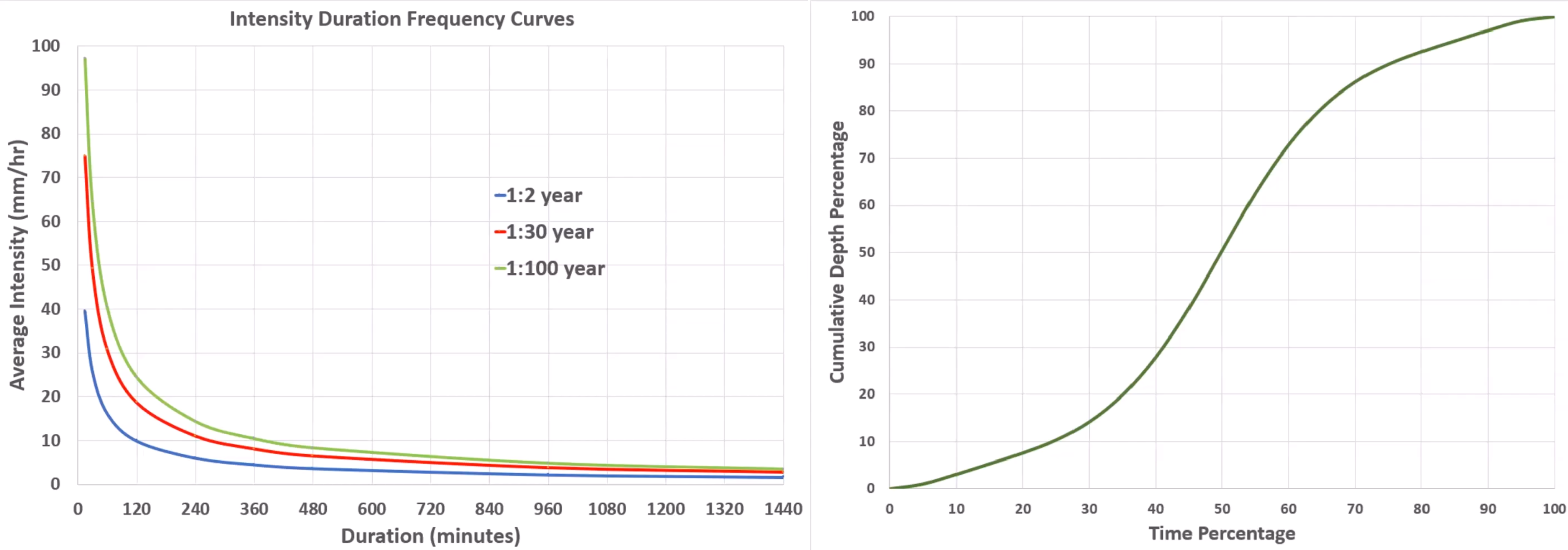
But to do so, you must be able to enter two pieces of information:

00:16

the IDF curve or curves,

00:19

and the dimensionless shape curve.

00:22

If you have data tables that reflect these, then you can build your own rainfall definition.

00:27

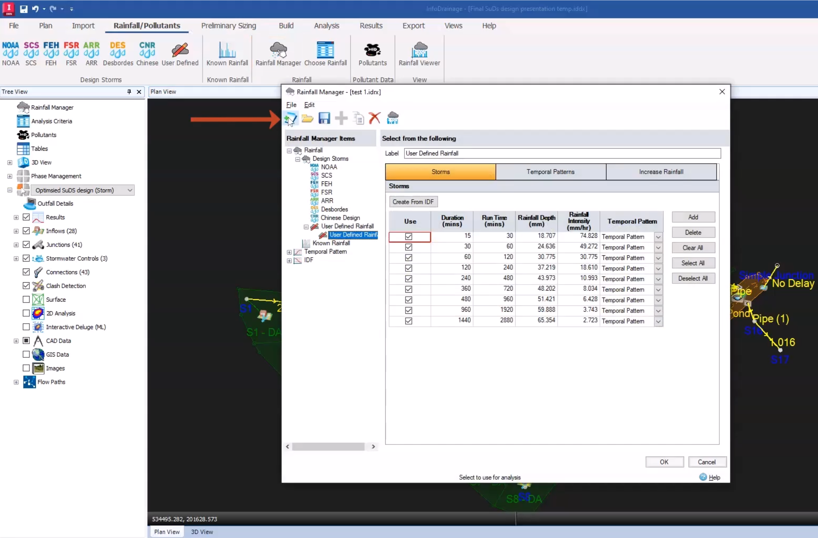
Open the Rainfall Manager, and in the toolbar, click New to create a new rainfall event.

00:34

For this example, name it “Test 1”, and then click Save.

00:39

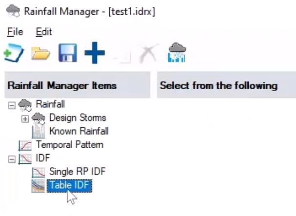
Under Rainfall Manager Items, expand the IDF node to access the IDF library.

00:46

If you had a single IDF curve, you would choose Single RP IDF.

00:51

But for this example, a series of curves is available in the spreadsheet,

00:56

so click Table IDF to create a table of events.

01:00

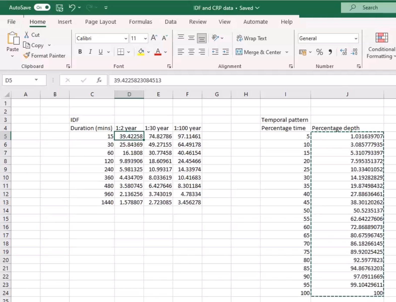
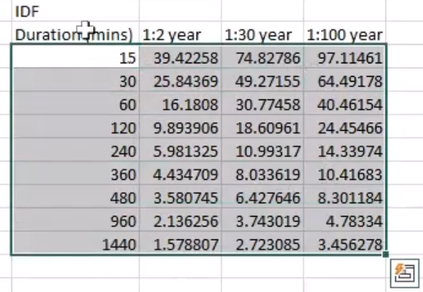
To review the data, open the sheet.

01:03

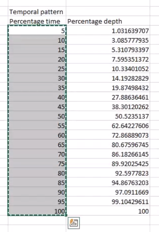
In this example, there are data for the IDF curves for three storm durations,

01:08

and temporal patterns for the dimensionless curve data.

01:12

Start with the IDF data.

01:15

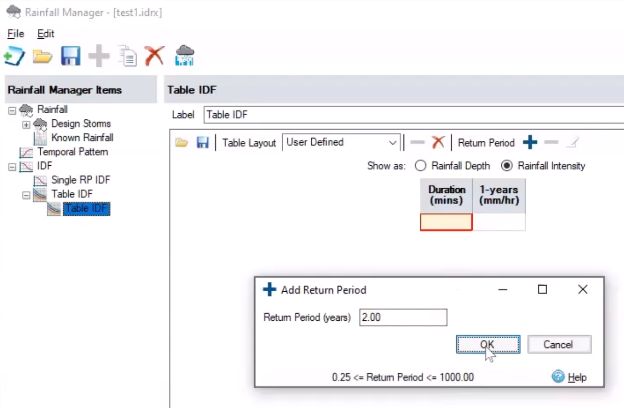
Back in the Rainfall Manager, with Table IDF selected, click Add.

01:21

First ensure that Rainfall Intensity is enabled to specify that you are entering rainfall intensity values.

01:29

Next, since the Duration already has a column,

01:32

you only need to create columns for each of the three return periods.

01:36

In the table tools, click Add (+).

01:40

In the Add Return Period popup, add in one of the return periods.

01:46

In the Return Period (years) field, enter 2, for the 2-year return period, and then click OK.

01:54

Repeat this process to add in the 30-year and then the 100-year return periods.

01:60

Back in the table in the Rainfall Manager,

02:04

you do not need the 1-year return period for this exercise,

02:07

so select the column header and then click Delete (-) to remove it.

02:11

Once the column headers are set,

02:14

return to the spreadsheet and copy out the data.

02:18

Ensure that you copy only the actual data, not the headers.

02:23

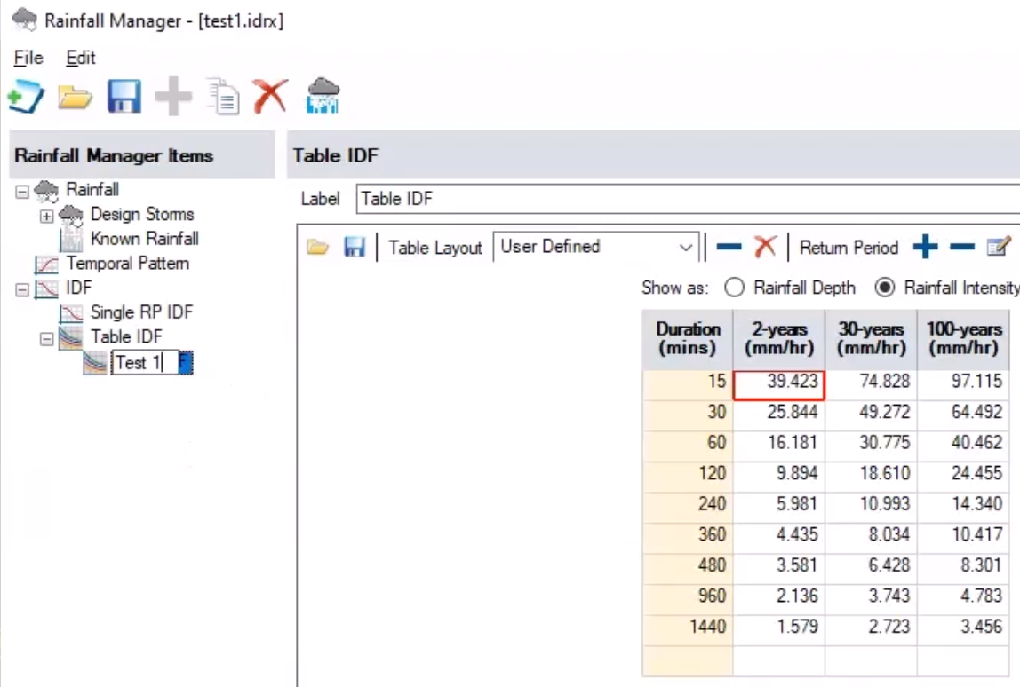
Back in the program, click the first cell under Duration,

02:27

and then paste the data.

02:29

With the three different return periods entered,

02:32

best practice is to rename the table.

02:35

Under the Items list, highlight the child Table IDF item,

02:38

and then type “Test 1” to rename it to match the project name.

02:43

Next, you need to enter the temporal pattern data,

02:47

which again is the dimensionless relationship data that defines the curve.

02:52

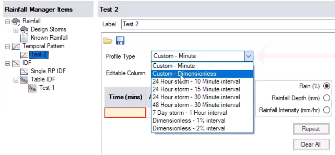
In the Rainfall Manager Items list, click Temporal Pattern.

02:56

Then in the toolbar, click Add (+).

02:59

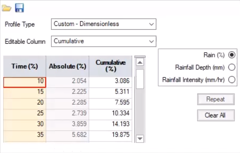
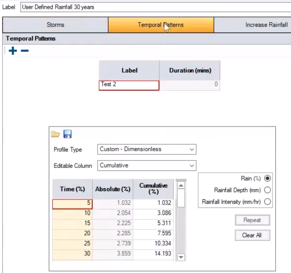
Under Temporal Pattern, next to Label, enter a name, such as “Test 2” for this exercise.

03:06

Expand the Profile Type drop-down and select Custom – Dimensionless.

03:12

For the Editable Column drop-down, keep Cumulative selected.

03:17

Back in the spreadsheet, copy the percentage time values, and again, do not include the header.

03:24

Be aware that for these, you cannot start from a percentage time of 0.

03:29

Copy from a non-zero value, such as 5, as shown here, through 100,

03:35

then place them into the table in the Rainfall Manager under Time (%).

03:40

Repeat this process with the Cumulative column.

03:43

From the spreadsheet, copy the data under Percentage depth,

03:47

then return to the program to paste it under Cumulative (%).

03:52

Now that you have the two essential elements—the IDF curve and the shape of the event—you need to bring them together

03:58

to create a series of user-defined rainfall events.

04:02

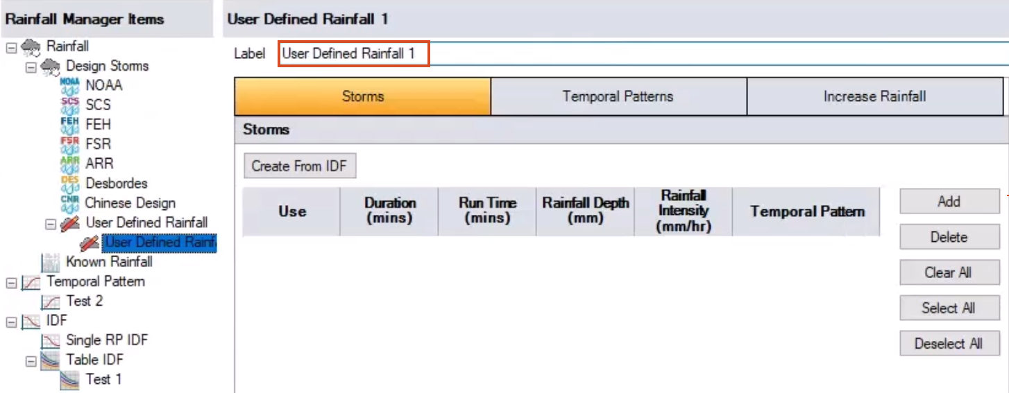
Expand the Design Storms node,

04:05

then select User Defined Rainfall.

04:08

Click Add (+).

04:11

Next to Label, rename it “User Defined Rainfall 1”.

04:16

Click OK to close the Rainfall Manager.

04:19

Note that for the library to update with the new information you just entered,

04:23

the Rainfall Manager first needs to close.

04:27

Now, when you re-open it, the User Defined Rainfall 1 Design Storm is still active,

04:32

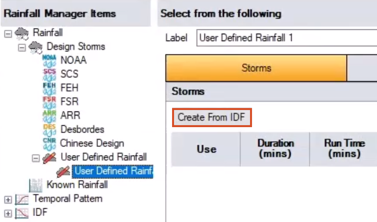
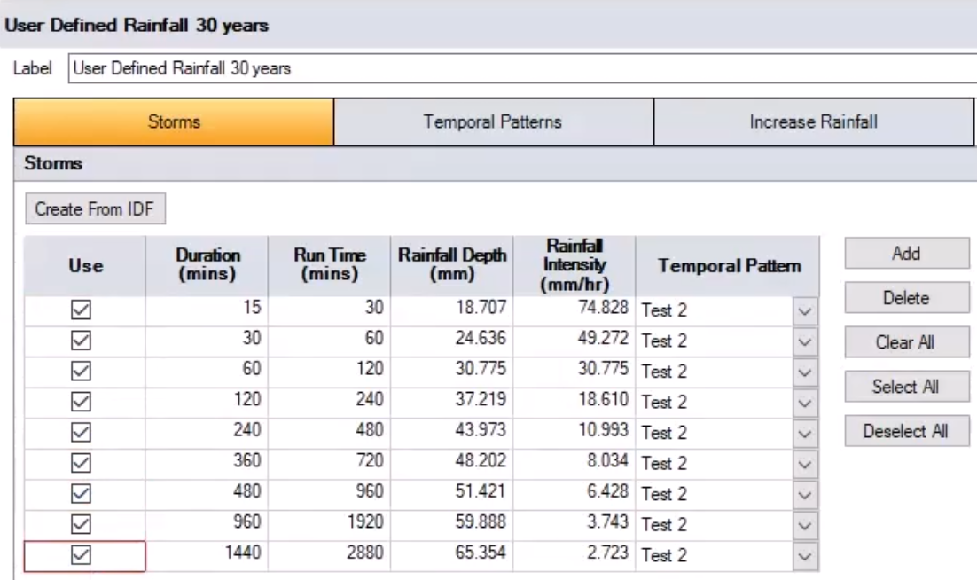
and on the Storms tab, notice that the Create From IDF tool is available.

04:37

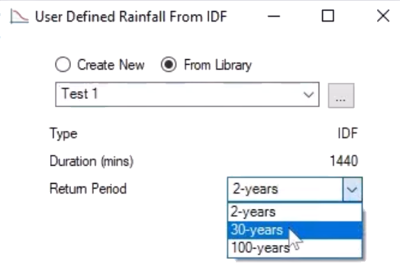
Click Create From IDF, and in the User Defined Rainfall From IDF popup,

04:42

select From Library, and then expand the drop-down.

04:47

The Test 1 IDF curve you created now appears in the library.

04:51

Select Test 1.

04:53

The return period information appears.

04:56

Expand the Return Period drop-down and select 30-years.

05:01

Click OK.

05:04

To identify it more clearly, change the Label to “30 years”, and then press ENTER.

05:10

Next, in the table, under Temporal Pattern, expand each drop-down and select the Test 2 pattern you created.

05:19

Ensure that you apply it to each one.

05:22

Also, enable Use for all the rows,

05:24

as it is not active by default.

05:27

This means you will now use these nine rainfall events

05:30

with the Temporal Pattern set to Test 2.

05:34

Click the Temporal Pattern tab, where you can double-check that it displays the data you entered.

05:39

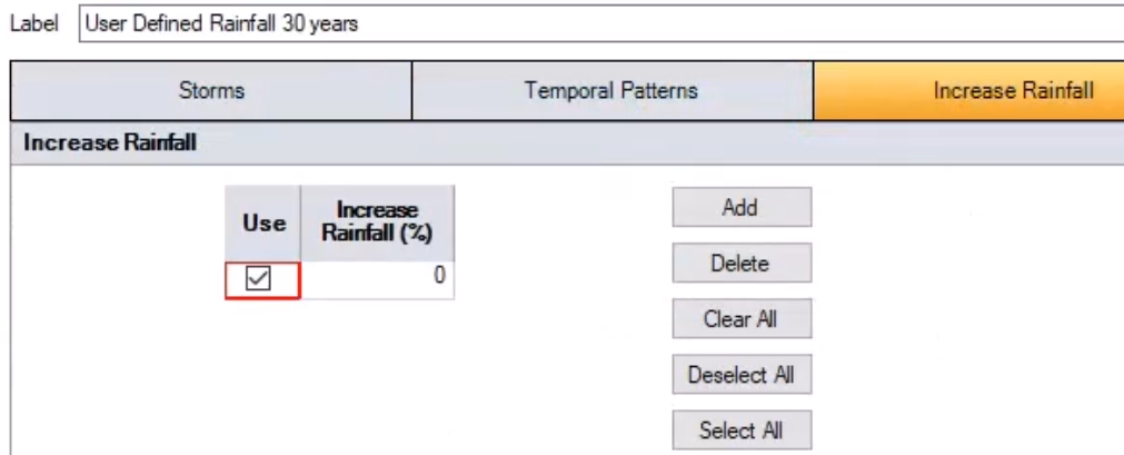
Click the Increase Rainfall tab.

05:42

If you wanted to add in an aspect of climate change, you could do that here.

05:47

Click Save to save your rainfall definition,

05:50

then click OK to close the Rainfall Manager.

05:54

Be aware that you can reuse this same rainfall later, if needed.

05:59

Now, you can run an analysis using your data.

06:03

On the ribbon, Analysis tab, Criteria panel, click Analysis Criteria.

06:10

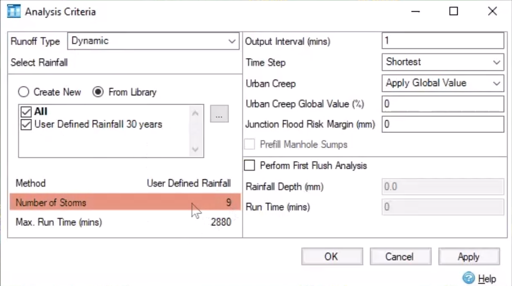
In the Analysis Criteria dialog,

06:13

your User Defined Rainfall 30 years set of curves is now available.

06:18

And crucially, you can see that there are nine rainfall events matching the nine that you chose to use.

06:24

Click OK.

06:26

It is always good practice to run a validation,

06:30

so in the ribbon, click Validate.

06:33

In the Validate dialog, if it shows as OK, click OK to close it.

06:38

In the ribbon, click Go.

06:42

A Progress dialog appears.

06:44

This network model is small, with only 40 manholes and 40 pipes, and only 9 storms.

06:51

This does not take long to process, but a larger model may take longer.

06:57

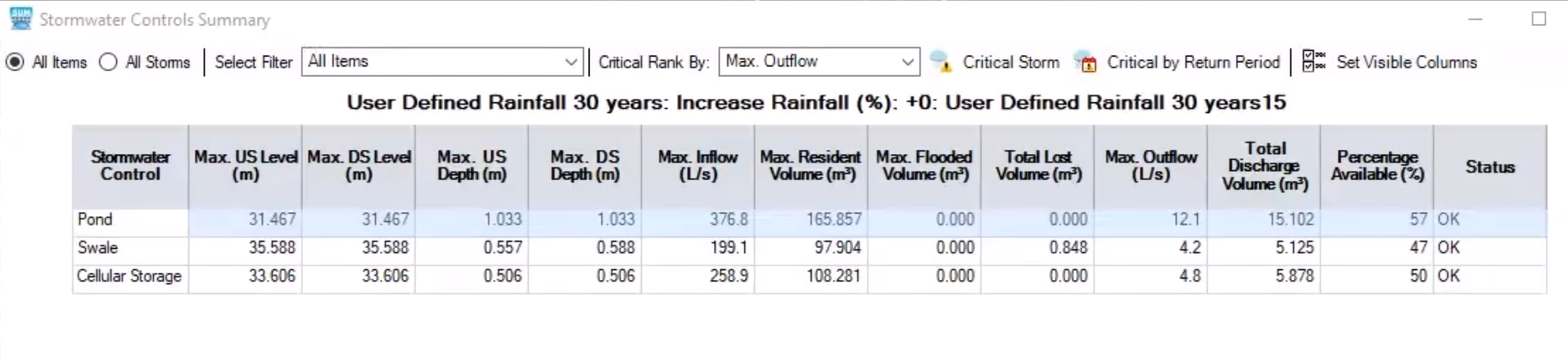
Once the simulation is finished, the Stormwater Controls Summary appears,

07:01

but you can look at the results in several different ways.

07:05

Click Close.

07:07

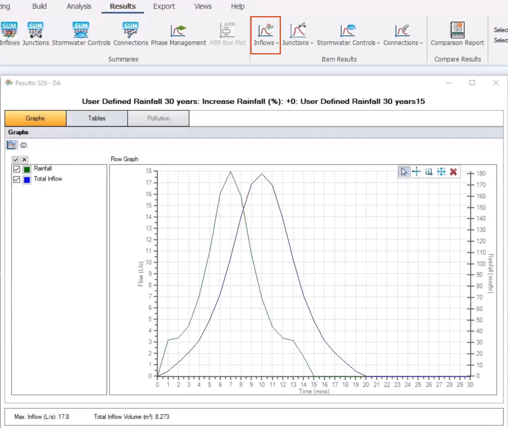
For example, on the ribbon, click the Results tab,

07:11

and in the Item Results, expand the Inflows drop-down and select S29-DA.

07:18

In the graph, you can look at the flows entering or leaving an inflow area, or entering a manhole.

07:24

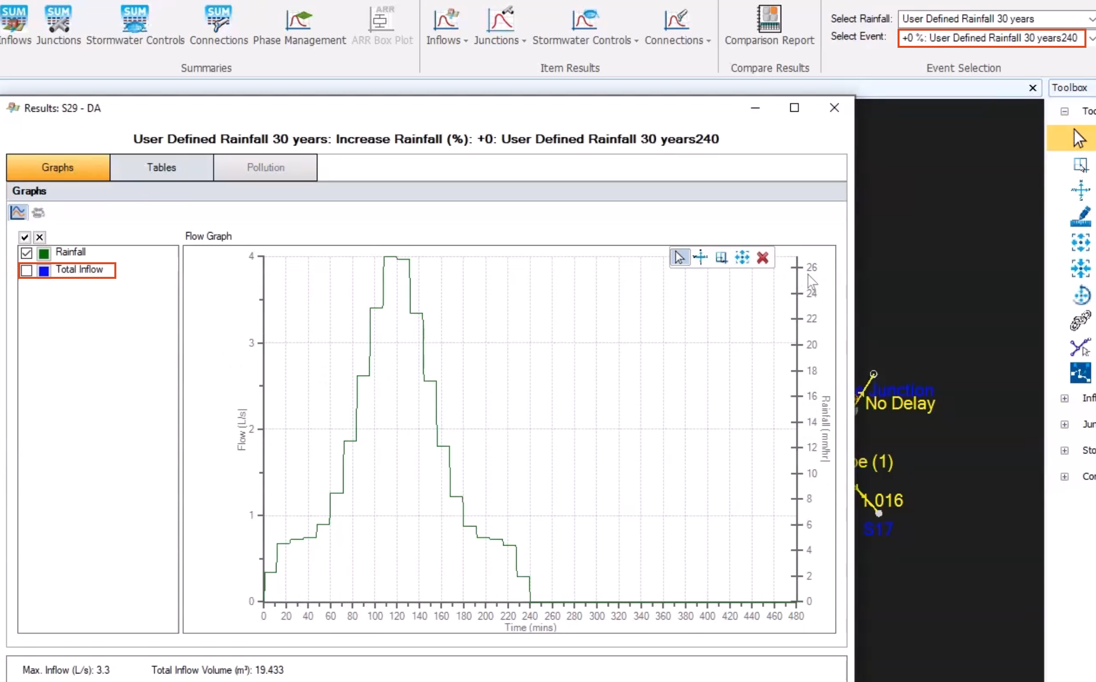
You can also choose which rainfall events you want to review.

07:29

In the Event Selection panel, expand the Select Event drop-down

07:33

and choose a different rainfall event, such as 240.

07:37

Back in the graph, if you switch off the inflow, you can see only the rainfall.

07:42

In this case, because it is a 1-in-30-years storm, 240-minute event,

07:47

the maximum intensity is a little more than 26 millimeters per hour.

07:53

As you can see, creating your own rainfall data for determining temporal patterns is easy

07:58

if you have the IDF curve and shape curve data for your area of interest.