Working with demand area expected leakage

00:04

In info works.

00:05

WS pro a demand area analysis provides data that allows users to

00:09

review the current demand for water and project future potential demand areas.

00:15

After generating demand areas from area codes with the demand area grid open,

00:20

you can view and edit the parameters of the

00:22

expected leakage calculation and review the results of the calculation

00:26

from the grid right click demand area 35 and select properties.

00:31

The demand area 35 dialog box appears which

00:34

contains the properties for this specific demand area

00:38

to view the results as a graph open the expected leakage tab

00:44

the infrastructure correction factor ICF field displays a factor

00:47

that indicates the relative condition of the mains.

00:51

The expected range is between 0.1 and two where

01:01

The pressure correction factor PCF field displays a factor that is used to correct

01:06

the AZN P or average zone night pressure to a standard 50 m.

01:12

The expected range is between 0.1 and three.

01:16

If a default value is chosen,

01:18

then the value of the PCF will be

01:20

calculated according to the chosen leakage index method.

01:25

The value for A

01:26

and P is taken from live data where available.

01:29

Otherwise the simulation results will be used.

01:33

The leakage index method uses either leakage indices or

01:36

the 1.5 Power Law to calculate the pressure correction factor

01:41

in the table.

01:41

Both background losses and equivalent service pipe bursts are

01:45

calculated using the infrastructure and pressure correction factors.

01:49

The number of props and the length of mains

01:52

reviewing expected leakage calculations allows you to ensure reliable and

01:57

efficient service across all points within a demand area.

Video transcript

00:04

In info works.

00:05

WS pro a demand area analysis provides data that allows users to

00:09

review the current demand for water and project future potential demand areas.

00:15

After generating demand areas from area codes with the demand area grid open,

00:20

you can view and edit the parameters of the

00:22

expected leakage calculation and review the results of the calculation

00:26

from the grid right click demand area 35 and select properties.

00:31

The demand area 35 dialog box appears which

00:34

contains the properties for this specific demand area

00:38

to view the results as a graph open the expected leakage tab

00:44

the infrastructure correction factor ICF field displays a factor

00:47

that indicates the relative condition of the mains.

00:51

The expected range is between 0.1 and two where

01:01

The pressure correction factor PCF field displays a factor that is used to correct

01:06

the AZN P or average zone night pressure to a standard 50 m.

01:12

The expected range is between 0.1 and three.

01:16

If a default value is chosen,

01:18

then the value of the PCF will be

01:20

calculated according to the chosen leakage index method.

01:25

The value for A

01:26

and P is taken from live data where available.

01:29

Otherwise the simulation results will be used.

01:33

The leakage index method uses either leakage indices or

01:36

the 1.5 Power Law to calculate the pressure correction factor

01:41

in the table.

01:41

Both background losses and equivalent service pipe bursts are

01:45

calculated using the infrastructure and pressure correction factors.

01:49

The number of props and the length of mains

01:52

reviewing expected leakage calculations allows you to ensure reliable and

01:57

efficient service across all points within a demand area.

Video quiz

Reviewing Expected Leakage for demand area analysis allows you to do which of the following?

(Select one)
Select an answer

1/1 questions left unanswered

Step-by-step Guide

In InfoWorks WS Pro, a demand area analysis provides data that allows users to review the current demand for water and project future potential demand areas.

To view and edit the parameters of the expected leakage calculation:

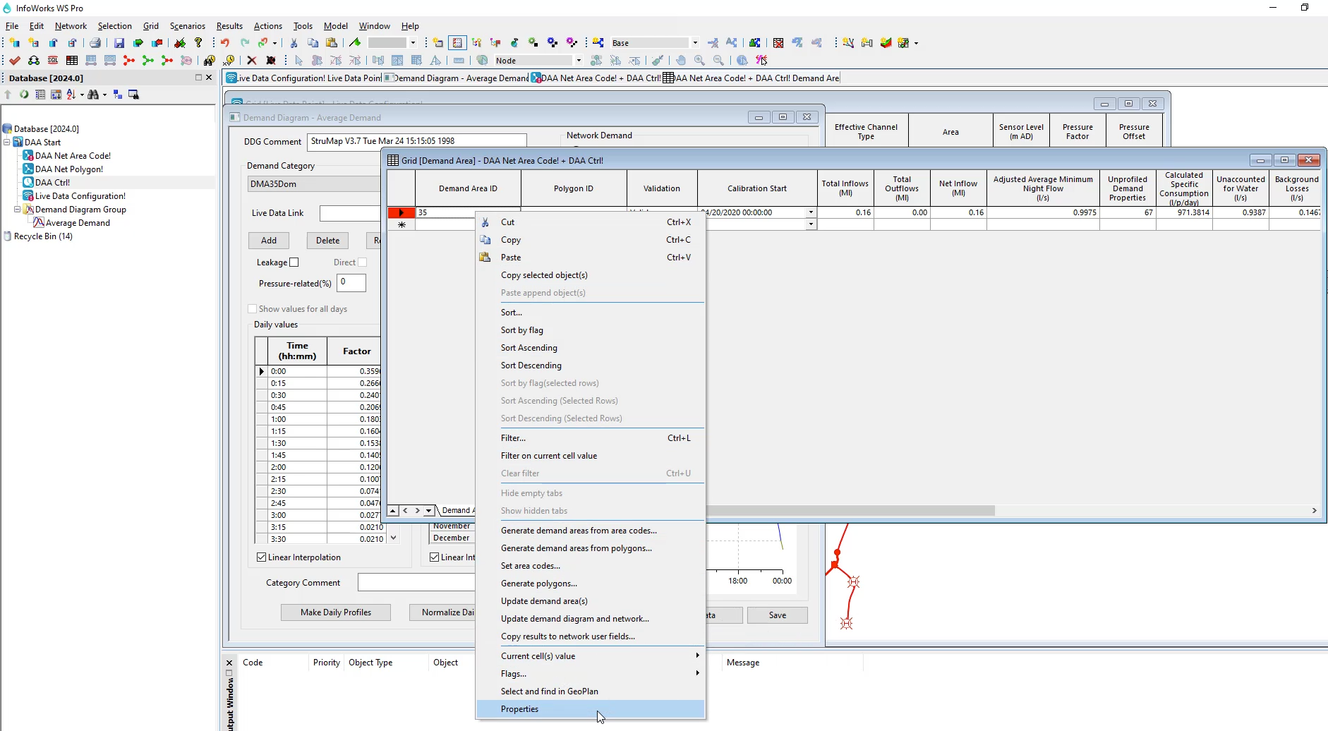
  1. Open the Demand Area Grid.
  2. Right-click Demand Area 35 and select Properties.

In the InfoWorks WS Pro interface, the Demand Area Grid with the shortcut menu for Demand Area 35 displayed and Properties selected.

  1. In the properties dialog box, open the Expected Leakage tab.

The properties dialog box for Demand Area 35, with the Expected Leakage tab open and highlighted in red.

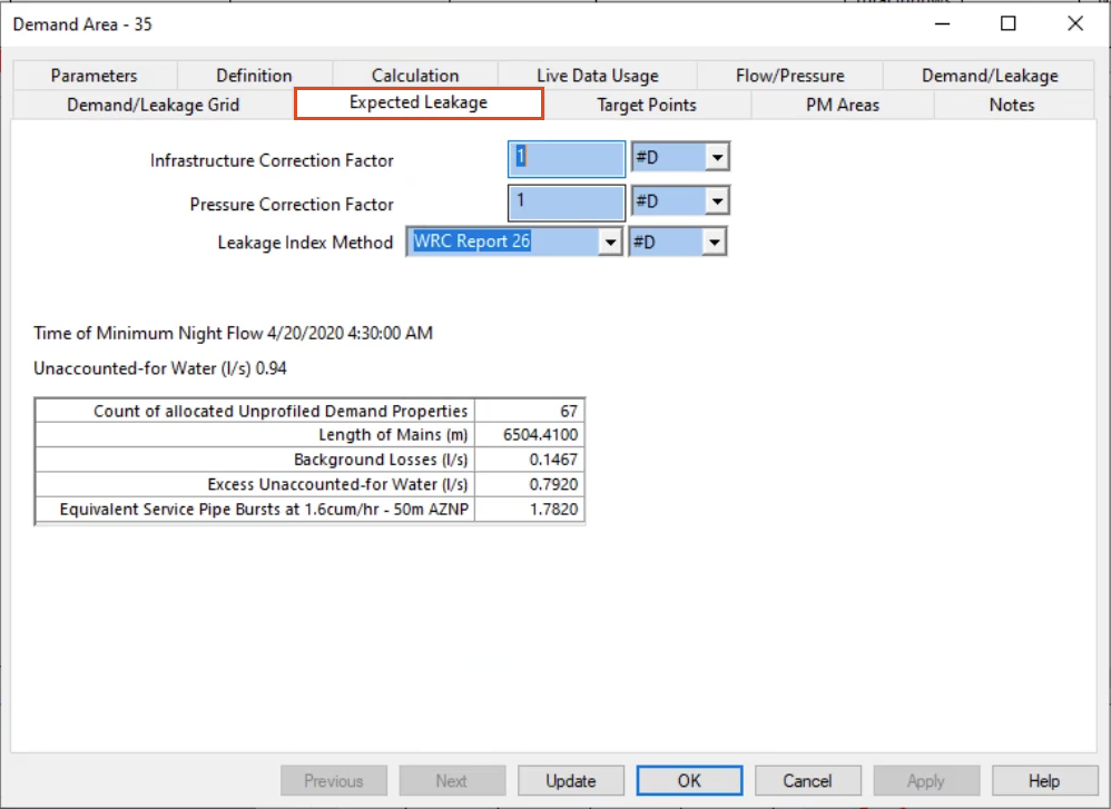
    • The Infrastructure Correction Factor (ICF) field displays a factor that indicates the relative condition of the mains. The expected range is between 0.1 and 2, where 0.1 indicates a good condition and 2 indicates poor.
    • The Pressure Correction Factor (PCF) field displays a factor that is used to correct the AZNP, or average zone night pressure, to a standard 50m. The expected range is between 0.1 and 3. If a default value is chosen, then the value of the PCF will be calculated according to the chosen Leakage Index Method. The value for AZNP is taken from live data where available. Otherwise, the simulation results will be used.
    • The Leakage Index Method uses either leakage indices or the 1.5 Power Law to calculate the Pressure Correction Factor.
    • In the table, both Background Losses and Equivalent Service Pipe Bursts are calculated using the infrastructure and pressure correction factors, the number of props, and the lengths of mains.
Was this information helpful?