Architecture, Engineering
& Construction
& Construction

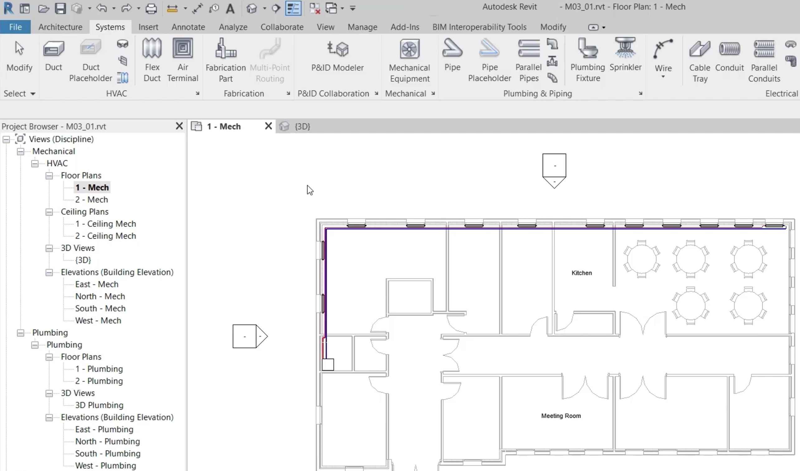
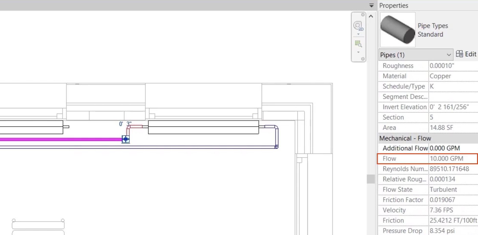
Integrated BIM tools, including Revit, AutoCAD, and Civil 3D
Top products
Product Design
& Manufacturing
& Manufacturing

Professional CAD/CAM tools built on Inventor and AutoCAD
Top products